
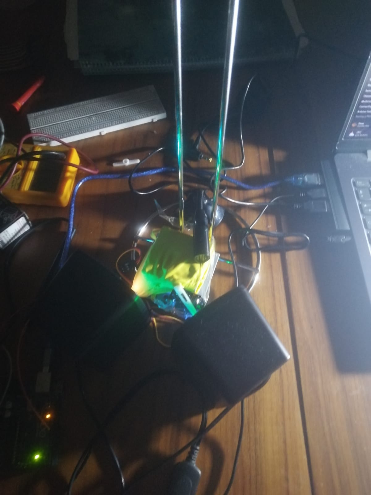
Acoustic metamaterials can be programmed by mechanically altering their boundary conditions. In this post, I’ll show how I used Python and Arduino to control a cube with a servo motor, excite it with a 50 Hz tone, record its resonance, and classify its spectral fingerprints into symbolic logic outputs.
UNSTRETCHED or STRETCHED) to Arduino.
import serial, time
import sounddevice as sd
import numpy as np
from scipy.signal import find_peaks

ser = serial.Serial('COM3', 115200)
fs = 44100
duration = 5.0
excitation_freq = 50.0

# Excitation signal
t = np.linspace(0, duration, int(fs*duration), endpoint=False)
signal = np.sin(2*np.pi*excitation_freq*t)

def excite_and_record(label):
    ser.write((label + "\n").encode())
    time.sleep(2)
    print(f"Exciting cube at {excitation_freq} Hz in {label} mode...")
    recording = sd.playrec(signal, samplerate=fs, channels=1, dtype='float64')
    sd.wait()
    samples = recording.flatten()
    fft_vals = np.abs(np.fft.rfft(samples))
    freqs = np.fft.rfftfreq(len(samples), d=1/fs)
    peaks, _ = find_peaks(fft_vals, height=np.max(fft_vals)*0.2)
    peak_freqs = freqs[peaks]
    print(f"{label} peaks: {np.round(peak_freqs,1)} Hz")
    return peak_freqs

def classify_output(peaks):
    peaks = list(peaks)
    if any(9 < p < 14 for p in peaks) or any(30 < p < 36 for p in peaks):
        return "A"
    elif any(abs(p-50)<2 for p in peaks) and any(140 < p < 210 for p in peaks):
        return "C"
    elif any(abs(p-50)<2 for p in peaks):
        return "C"
    else:
        return "?"

while True:
    peaks_un = excite_and_record("UNSTRETCHED")
    code_un = classify_output(peaks_un)
    print(f"UNSTRETCHED logic output: {code_un}")
    time.sleep(5)
    peaks_st = excite_and_record("STRETCHED")
    code_st = classify_output(peaks_st)
    print(f"STRETCHED logic output: {code_st}")
    time.sleep(5)
- Unstretched mode often produces low-frequency clusters (≈12–33 Hz) → classified as A.
- Stretched mode produces strong 50 Hz + harmonics (≈150–200 Hz) → classified as C.
- Sometimes both states collapse to a single 50 Hz peak, still classified as C.
By running multiple cycles and plotting spectra, we can demonstrate repeatability. Here’s an example of overlaying multiple cycles:

Beyond the 50 Hz excitation, the cube shows a rich resonance landscape with multiple peaks between 80 Hz and 400 Hz. This broader spectrum highlights how stretching alters not just the fundamental mode but also higher harmonics.

This workflow turns a resonant cube into a programmable element: servo input → resonance fingerprint → symbolic logic output. By expanding the codebook and combining multiple cubes, you can build logic gates and analogue computing structures. This is a powerful way to explore how physical systems can be programmed through resonance.
To make the process more tangible, here’s a snapshot of the Python script running and classifying resonance peaks into logic outputs:

In this run, the cube alternated between modes, producing fingerprints such as [24.0, 50.0] Hz (classified as C) and
[11.6, 12.0, 12.6, 13.0, 20.6, 49.0, 50.0, 100.2, 150.2, 200.2, 300.2] Hz (classified as A).
This demonstrates how the cube’s resonance spectrum can be interpreted as programmable logic outputs in real time.
From servo control to FFT analysis, the resonant cube can be programmed to output symbolic codes based on its acoustic fingerprints. Adding live output screenshots alongside plots gives readers both the quantitative and experiential view of the experiment. This combination of hardware, software, and resonance analysis makes for a compelling blog post on programmable acoustic metamaterials.